Computer Algebra with Pure: A Reduce Interface

Version 0.4, April 11, 2018

Albert Graef <aggraef@gmail.com>

Kurt Pagani <kp@scios.ch>

One of Pure’s distinguishing features as a term rewriting programming language is that it makes the symbolic manipulation of expressions very easy and convenient. It is thus a natural environment for hosting a full-featured computer algebra system (CAS). Computer algebra systems are complex pieces of software featuring advanced algorithms for simplification of algebraic expressions, symbolic integration, equation solving and much more. Reimplementing all these algorithms in Pure would be a major undertaking, to say the least. A much better option is to interface to an existing CAS which has already proven its worth to the scientific computing community, has been tested extensively and is known to be both reliable and efficient.

This is also the approach taken by Pure’s reduce module which interfaces to the well-known Reduce system. Along with Macsyma/Maxima, Reduce is one of the oldest computer algebra systems which has been around since the 1960s and is widely recognized as a state-of-the-art, powerful and efficient CAS. It is free/open source software distributed under a BSD-style license, actively maintained on its SourceForge website, and implementations exist for all major computing platforms. The reduce module makes the functionality of Reduce available in Pure in a seamless way. It uses an “embedded” version of Reduce in the form of a shared library which is easy to build from the Reduce sources; the Installation section below describes how to do this. More background information and a discussion of the interface can be found in the Embedding REDUCE thread on the Pure mailing list.

The interface can be found in the reduce.pure module. It has two parts, a low-level interface which consists of a handful of C entry points supplied by the Reduce library, and a high-level interface which provides everything that the Pure programmer needs to use Reduce from Pure. Please note that at present this module is still experimental. But the basic functionality works, and you’re welcome to discuss the new interface on the mailing list and/or submit bug reports and patches.

Copying

pure-reduce is available under the same 2-clause BSD license as Reduce itself, please see the accompanying COPYING file and the reduce.pure file for details.

Installation

Get the latest source from https://bitbucket.org/purelang/pure-lang/downloads/pure-reduce-0.4.tar.gz.

You’ll need both the Reduce library (named reduce.so, reduce.dylib or reduce.dll, depending on the system you have) and a Reduce image file (reduce.img) to make this module work. A Makefile is included with this package so that you can build these yourself from the Reduce sources. (In principle, this only needs to be done once for the initial installation of this module, but you may want to repeat this procedure every once in a while to get the latest Reduce version.)

The full Reduce system is a big package, so we have packaged a stripped-down version of the Reduce source which contains all the bits and pieces needed to compile the Reduce library and image, and has also been patched up so that it compiles cleanly on recent Linux systems. At the time of this writing, you can find this package here:

https://bitbucket.org/purelang/pure-lang/downloads/reduce-algebra-csl-r2204.tar.bz2

(You may want to check the download section on the Pure website for newer revisions of this package, since we may update the package from time to time to the latest source from the Reduce svn repository.)

Unpack the reduce-algebra-csl tarball and move the resulting reduce-algebra directory into the pure-reduce source directory. Run make and then (if needed) make install in the pure-reduce directory (not in the reduce-algebra directory!). You should also run make check which performs a few tests in order to verify that the interface works ok (this can be done without installing the package, but needs the Reduce image and library).

For convenience, the Makefile also has a make reduce target which builds a minimal Reduce executable. If you use that option, make install installs this executable along with the library and image files, so that you can then run Reduce directly from the command line by just typing reduce. Please note that this is a really minimalistic Reduce frontend which is most useful for testing purposes. (If you want the full Reduce version then you can find binary Reduce packages for various systems at SourceForge. But note that neither the minimalistic nor the full Reduce frontend is required for the pure-reduce module in any way.)

It is also possible to build the Reduce library and image directly from the latest source in the Reduce svn repository. You can check out the repository with the following command:

svn co svn://svn.code.sf.net/p/reduce-algebra/code/trunk reduce-algebra

This pulls down many hundreds of megabytes, so this may take a while. Once the checkout is finished, you’ll end up with a reduce-algebra directory which you can drop into the pure-reduce source directory and proceed with the compilation as described above. Note that if you go that route then you should be prepared to deal with compilation problems in the Reduce sources. Reduce is a big and complicated software, so the svn sources are not always in a state which guarantees smooth compilation on all supported systems. If you run into problems then please consider using our streamlined reduce-algebra-csl package instead.

Low-Level Interface

The low-level interface is a straight wrapper of the C entry points provided by the Reduce library, also known as the “procedural” or PROC interface, for short. It uses an embedded version of Reduce which runs on a free and open-source Lisp flavour known as CSL (Codemist Standard Lisp). The external C routines are all declared in the reduce namespace. Normally you shouldn’t have to call these functions directly, since we provide a high-level, idiomatic Pure interface which makes calling Reduce from Pure much easier, see below.

High-Level Interface

The high-level interface provides a wrapper of the low-level PROC interface which makes calling Reduce from Pure easy and convenient. After installing the module, it can be imported in your Pure scripts as follows:

using reduce;

This starts up Reduce and makes the following variables and functions available in Pure.

Starting and Stopping Reduce

variable REDUCE_PATH

This variable holds a colon-delimited search path used to locate the Reduce image file (see reduce::start below). By default this includes the current directory and the Pure library directory.

reduce::start image::string args::smatrix

Initializes the Reduce system. This is done automatically when loading this module, so normally you shouldn’t have to call this manually, unless the default image file wasn’t found or you want to restart the Reduce system with your own image file or your own set of options. When calling this operation manually, you need to specify the name of the Reduce image file and any desired extra arguments as a string vector. Unless the filename contains a slash, reduce::start searches the directories in REDUCE_PATH for the image file. An exception is raised if the image file isn’t found.

reduce::finish

Finalizes the Reduce system. You can call this to release the resources of the Reduce system. (reduce::start also invokes this automatically if a Reduce instance is already running, so it isn’t necessary to call reduce::finish in this case.)

Maintenance Operations

reduce::verbosity n

Sets the verbosity level; 0 means no messages at all (which is the default when using this module), and the following values may be or’ed together to pick what you need:

1: messages whenever garbage collection happens

2: messages whenever a module of code is loaded

4: extra details in the garbage collector messages

reduce::switch name:string val::int

Lets you change global Reduce options. This works like Reduce’s on and off declarations; please check the Reduce documentation for details.

reduce::capture flag::int

reduce::output

Captures output from Reduce. If flag is nonzero, reduce::capture arranges for all output from Reduce to be buffered. The contents of the buffer can then be read using the reduce::output function which returns a string value. If flag is zero, capturing is disabled so that output goes to stdout again.

reduce::feed s::string

Feeds input to Reduce. Reduce will read input from the given string s, switching back to stdin after s has been processed.

reduce::load name::string

Loads Reduce packages. This works like Reduce’s load_package command; please check the Reduce documentation for details.

reduce::in name::string

Sources the given Reduce (.red) file. This works like the Lisp in function. Output is captured using reduce::capture, see above.

Evaluation

For convenience, the following operations are in the default namespace:

simplify x

This is the main entry point. It takes an algebraic expression in Pure format and tries to simplify it using Reduce. The result is then converted back to Pure format. Note that you need to quote x if you want to prevent it from being evaluated on the Pure side.

simplifyd x

A variation of simplify which takes care of customary mathematical notation for limits, integrals and differentials, so that you can write stuff like d f/d x and lim n inf (1/n) and have that expanded to the corresponding Reduce calls automatically. This also tries to support most of the idioms and variations of notation which can be seen in output of the Reduce tmprint module and which are commonly used in TeXmacs documents.

lisp x

This can be used to execute arbitrary Lisp code, which is sometimes necessary to perform special functions in the Reduce system. Note that you need to quote x if you want to prevent it from being evaluated on the Pure side. This is true, in particular, for the quote itself, which needs an extra level so that one quote goes through to the Lisp system (e.g.: lisp (''(a b c))). For convenience, free symbols are quoted automatically, and Pure lists are mapped to corresponding Lisp lists and vice versa (so lisp [a,b,c] actually yields the same result as lisp (''(a b c))). The result is always a Pure list or an atomic value.

lispval x

This converts a Pure expression to its Reduce equivalent, like simplify does, but without actually simplifying it. As with the other functions, you need to quote x if you want to prevent it from being evaluated on the Pure side. The result is the Pure representation of a Lisp form which can be passed as a value to other Lisp routines by employing the lisp function. (Normally this requires that you double-quote the expression so that it doesn’t get evaluated by the Lisp interpreter.) This function isn’t for casual usage, but may be useful if you need to pass a Reduce expression to some Lisp function which cannot be called through simplify.

lispsym s::string

This function creates a special Pure identifier for any symbol given as a string, even symbols which don’t conform to Pure syntax. This is sometimes needed to specify special Lisp symbols in calls to lisp, such as lisp (lispsym "oem-supervisor"). (Note that if such a special symbol occurs as a literal in a result returned by lisp or simplify then it will get mangled into a form which conforms to Pure syntax.)

declare declsym [foo,bar,...]

Declare symbols and their properties; please see the Declarations section in the Reduce manual for details. The second argument can also be a singleton symbol. In the present implementation, declsym must be one of:

• operator: declares an operator symbol;
• precedence: declares an infix operator and optionally specifies its precedence (giving the symbol priority over a second given symbol);
• antisymmetric, symmetric, even, odd, linear, noncom and nonzero: declares properties of already declared operator symbols;
• depend, nodepend, factor, remfac, order, korder: declares kernel dependencies and orders. These take both symbols and “kernels” as arguments (the latter are simple prefix expressions which denote irreducible subterms such as cos x; Reduce treats these more or less like variables in algebraic simplifications).

precision prec::int

Sets the internal Reduce precision in decimal digits for floating point calculations, and returns the previously set precision. This takes effect when rounded mode is enabled (reduce::switch "rounded" 1). Note that at present this only affects Reduce’s internal precision, floating point values are still returned as double precision numbers in Pure land.

plotreset

This is identical to the plotreset command provided by Reduce’s gnuplot interface, and is sometimes needed to reset the plot subsystem.

In Pure land, Reduce expressions are represented using Pure’s standard curried notation. Marshalling of numeric data works in a straightforward fashion and includes all natively supported Pure data types (machine ints, bigints, doubles, rationals and complex numbers). Some special conversions are applied to algebraic expressions to make arithmetic operations such as +, * etc. work as expected. In addition, the ==, =>, .. and := infix operators can be used to denote equations, replacement rules, ranges and assignments in Reduce, respectively. (Note that you may have to quote these in some cases so that they don’t get evaluated on the Pure side.) Also, Reduce’s arbconst n, arbint n and arbcomplex n terms can be mapped to Greek symbols αn, βn and ζn on the Pure side. (This may cause issues in environments without proper Unicode support, so it’s disabled by default.) For debugging purposes, all these automatic conversions can also be turned off on the output side with the ‘#!  --disable mapped‘ compilation pragma; this needs to be placed before the ‘using reduce;‘ import clause to take effect. There are a number of other conditional compilation options which may be used to selectively turn off some of the conversions; please check the module source for details.

Lisp expressions are handled in a similar fashion, but here only a few basic Pure data types (integers, doubles, strings and lists) are converted to and from corresponding Lisp data. Function applications in Pure’s curried notation are mapped to corresponding Lisp forms. The result of invoking lisp is always one of the supported atomic types or a Pure list.

The lisp function is to be used with care. An orderly Pure exception is raised if you try to execute a non-existing Lisp function. But there are some internal functions in Reduce which aren’t very forgiving if you try to execute them with invalid arguments, and will most likely crash the Reduce system in such cases. You have been warned!

Basic Examples

Here is a simple example showing how to start up Reduce and do some calculations:

> using reduce;
Reduce (Free CSL version), 27-Sep-12 ...
> simplify $ df ((x+5)^3) x;
3*x^2+30*x+75
> simplify $ intg (exp (2*x)) x;
e^(2*x)/2
> simplify $ solve (x^2+7) x;
[x==sqrt 7*i,x==-sqrt 7*i]

Note that the result returned by simplify is always a quoted expression. If the expression can be further reduced on the Pure side, you’ll have to use Pure’s eval function to force its evaluation:

> using math;
> eval ans;
[x==0.0+:2.64575131106459,x==0.0+:-2.64575131106459]

The following example shows how you can do a simple plot using Reduce’s gnuplot module:

> simplify $ plot [sin x/x, x=='(-20..20), terminal=="wxt"];
0

This pops up a wxWidgets window (terminal=="wxt") with a plot of the given function in it, see the screenshot below. The x=='(-20..20) argument specifies the desired range of the x variable (note that the range needs to be quoted so that it gets through to Reduce rather than being evaluated on the Pure side).

Reduce gnuplot example.

The same plot can be written to a PostScript file sinc.ps as follows:

> simplify $ plot [sin x/x, x=='(-20..20), terminal=="postscript", output=="sinc.ps"];
0

The lisp function can be used to execute Lisp code in the CSL interpreter hosting the Reduce system. Here are some basic examples. Note that, to be on the safe side, we just always quote the argument to lisp here to prevent its evaluation on the Pure side.

> lisp ('plus 2 3);
5
> lisp ('car (list a b c d e));
a
> lisp ('cdr [a,b,[c,d],e]);
[b,[c,d],e]

Lisp’s truth values are t and nil; the latter is just the empty list, so that’s what you get if a Lisp predicate evaluates to “false”:

> lisp ('lessp 5 3);
[]
> lisp ('greaterp 5 3);
t

Most simple kinds of Lisp calls should be doable that way, but don’t expect any miracles; the lisp function is provided to access special functionality in the “symbolic mode” of the Reduce system, not to turn Pure into a full-featured Lisp frontend. The following example illustrates how you can use the lisp function to declare an operator symbol and change or query its properties:

> lisp ('operator [myop]);
[]
> lisp ('flag [myop] odd);
[]
> lisp ('prop myop);
[odd:t,simpfn:simpiden]
> simplify (myop (-x));
-myop x

If you find it awkward to evaluate Lisp forms in Pure, you can also achieve the same with the declare function which covers most of the common Reduce declarations that might be needed:

> declare operator myop;
[]
> declare odd myop;
[]
> simplify (myop (-x));
-myop x

For basic Pure-based usage of Reduce, it’s convenient to have a simple read-eval-print loop which lets you type some declarations and expressions to be simplified (in Pure syntax), and takes care of all the quoting and invoking simplify for you. Here’s a little Pure script which does that:

using math, reduce, system;

/* You might want to replace this with the real readline if you have the
   corresponding Pure module installed. See the red.pure script in the
   distribution for details. */
myreadline prompt::string = fputs prompt stdout $$ fflush stdout $$ gets;

red = loop with
  // A simplistic REPL.
  loop = case myreadline "> " of
    s::string = process s $$ loop if ~null s;
    _ = () otherwise;
  end;
  // Get rid of trailing blanks and semicolons.
  process s = process (init s) if any (==last s) [" ",";"];
  // Process a declaration or REDUCE expression.
  process s = case val s of
    val _ = fputs "** syntax error\n" stderr if ~null lasterr;
    on flag = reduce::switch (str flag) 1;
    off flag = reduce::switch (str flag) 0;
    x@(declare _ _) = eval x;
    x = puts (str (simplify x)) otherwise;
  end;
end;

Now you can run red at the Pure prompt and start typing the stuff you want to evaluate, one expression or declaration per line. Enter an empty line or Ctrl-D when you’re done to return to the Pure command prompt.

> red;
> df ((x+5)^3) x
3*x^2+30*x+75
> intg (exp (2*x)) x
e^(2*x)/2
> on rounded
> solve (x^2+7==17) x
[x==3.16227766016838,x==-3.16227766016838]
> off rounded
> solve (x^2+7==17) x
[x==sqrt 10,x==-sqrt 10]
> declare operator myop
> declare odd myop
> myop (-x)
-myop x
> plot [sin x/x, x==(-20..20), terminal=="wxt"]
0
> ^D
()

Note that we barely scratched the surface here; Reduce is a very complex system with lots of capabilities. The following section explores some of these areas in more detail.

Examples by Topic

This is a small excerpt from the REDUCE User’s Manual [REDUM], translated to Pure syntax. For any details we refer to that document. With this guide it should be straightforward to translate back and forth between Pure and REDUCE syntax for the invocation of REDUCE functions. The one thing you have to keep in mind is that Pure uses curried notation for function applications, so where a function is invoked as f(x,y,z) in REDUCE, you’ll have to call it as f x y z in Pure (with parentheses around each argument which is a compound expression).

The REDUCE User’s Manual as well as the documentation of each package and other valuable information may be found at: http://www.reduce-algebra.com/documentation.htm

Differentiation

The operator df is used to represent partial differentiation with respect to one or more variables.

df exprn [var <num>]+

Differentiation of the function with respect to , two, three and four times respectively, i.e :

> simplify $ df (x^2*y^3*z^4) x 2 y 3 z 4 ;
288

The derivative of :

> simplify $ df (log(sin x)^2) x;
2*cos x*log (sin x)/sin x

Note the parentheses.

Suppose . Let’s calculate and :

> declare depend [z,cos x,y];
[]
> simplify (df (sin z) (cos x));
cos z*df z (cos x)
> simplify (df (z^2) x);
2*df z x*z

Note how to declare dependencies.

The results are and , respectively, as expected.

Integration

INT is an operator in REDUCE for indefinite integration using a combination of the Risch-Norman algorithm and pattern matching.

intg exprn var

Note that in Pure the operator is called intg in order not to clash with the int conversion function.

Example 1:

> simplify $ intg (1/(a*x+b)) x;
log (a*x+b)/a

Example 2:

> I a b n = simplify $ intg (x^2*(a*x+b)^n) x;
> I a b n;
((a*x+b)^n*a^3*n^2*x^3+3*(a*x+b)^n*a^3*n*x^3+2*(a*x+b)^n*a^3*x^3+
 (a*x+b)^n*a^2*b*n^2*x^2+(a*x+b)^n*a^2*b*n*x^2-2*(a*x+b)^n*a*b^2*
  n*x+2*(a*x+b)^n*b^3)/(a^3*n^3+6*a^3*n^2+11*a^3*n+6*a^3)
> I a b 0 ;
x^3/3
> I 0 b n;
b^n*x^3/3
> I a 0 k;
x^k*a^k*x^3/(k+3)

Example 3:

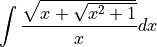
> simplify $ intg (sqrt(x+sqrt(x^2+1))/x) x ;
intg (sqrt (sqrt (x^2+1)+x)/x) x

Apparently no solution was found. There is a package ALGINT in REDUCE which specifically deals with algebraic functions. The REDUCE User’s Manual [REDUM] says:

This package [...] will analytically integrate a wide range of expressions involving square roots where the answer exists in that class of functions. It is an implementation of the work described in J.H. Davenport [LNCS102].

> reduce::load "algint" ;
0
> simplify $ intg (sqrt(x+sqrt(x^2+1))/x) x ;
atan ((sqrt (sqrt (x^2+1)+x)*sqrt (x^2+1)-sqrt (sqrt (x^2+1)+x)*x-sqrt
(sqrt (x^2+1)+x))/2)+2*sqrt (sqrt (x^2+1)+x)+log (sqrt (sqrt
(x^2+1)+x)-1)-log (sqrt (sqrt (x^2+1)+x)+1)

Note how to load packages.

Length, Map and Select

LENGTH is a generic operator for finding the length of compound objects. Besides lists and matrices, this also includes algebraic expressions. The MAP and SELECT operators let you manipulate such objects by applying a function to each element of the structure, or by picking the elements satisfying a given predicate function. Thus these operations serve pretty much the same purposes as # (or dim), map and filter in Pure, but in REDUCE they also work with the operands of an algebraic expression.

length exprn

map fun exprn

select fun exprn

> simplify $ length (a+b);
2
> simplify $ length (x^n+a*x+2);
3

> simplify $ 'map sqrt [1,2,3];
[1,2^(1/2),3^(1/2)]
> simplify $ 'map log  [x^n,x^m,sin x];
[log (x^n),log (x^m),log (sin x)]

Note that map must be quoted if we want to evaluate it in REDUCE, since it’s also a function in Pure. In this case, we might as well do the calculation using Pure’s map; the result is exactly the same.

> simplify $ map sqrt [1,2,3];
[1,2^(1/2),3^(1/2)]
> simplify $ map log  [x^n,x^m,sin x];
[log (x^n),log (x^m),log (sin x)]

If the function to be applied in calls to MAP or SELECT is a compound expression, it must either contain a single free variable (indicated with the ~ prefix, e.g.: ~w) or a replacement rule of the form var => exprn. In either case the current elements are substituted for the free variable when the function is applied.

> simplify $ 'map (y=>df y x)   [x^n,x^m,sin x];
[x^n*n/x,x^m*m/x,cos x]
> simplify $ 'map (y=>intg y x) [x^n,x^m,sin x];
[x^n*x/(n+1),x^m*x/(m+1),-cos x]

> simplify $ select (evenp (deg (~w) y)) ((x+y)^5);
x^5+10*x^3*y^2+5*x*y^4
> simplify $ select (w=>evenp (deg w y)) ((x+y)^5);
x^5+10*x^3*y^2+5*x*y^4

Contrast this with Pure where the function argument to map is often specified as a lambda:

> simplify $ map (\y->df y x)   [x^n,x^m,sin x];
[x^n*n/x,x^m*m/x,cos x]
> simplify $ map (\y->intg y x) [x^n,x^m,sin x];
[x^n*x/(n+1),x^m*x/(m+1),-cos x]

In principle, the same correspondences also hold between REDUCE’s select and Pure’s filter. For instance, consider:

> simplify $ select (w=>evenp (deg w x)) [2*x^2,3*x^3,4*x^4];
[2*x^2,4*x^4]

The equivalent Pure filter is:

> filter (\w->simplify $ evenp (deg w x)) [2*x^2,3*x^3,4*x^4];
[2*x^2,4*x^4]

Note that REDUCE is now being called inside the predicate function, the rest of the processing is done in Pure.

Of course, if you want to apply map, filter and similar Pure functions to an algebraic expression, you’ll first have to extract its components as a list. Here’s a little Pure function which mimics the way in which MAP and SELECT decompose an expression:

terms x = case x of
  f@_ u v = collect f x with
    // Collect the operands of variadic Reduce operators.
    collect f (f@_ u v) = collect f u+collect f v;
    collect f x = [x] otherwise;
  end if any (===eval f) [(+),(-),(*),min,max];
  = [u,v] if arity f == 2;
  _ = [x] otherwise;
end;

For instance, consider:

> simplify $ 'map (w=>w+1) (df ((x+y)^3) x);
3*x^2+6*x*y+3*y^2+3

With the help of terms we can also do this using Pure’s map as follows:

> map (+1) $ terms (simplify (df ((x+y)^3) x));
[3*x^2+1,6*x*y+1,3*y^2+1]
> simplify $ foldl (+) 0 ans;
3*x^2+6*x*y+3*y^2+3

While the REDUCE version is shorter and only involves a single call to simplify, with a little bit of programming the Pure solution can be made just as convenient. More importantly, this method easily generalizes to other list operations. This makes it possible to apply Pure’s full arsenal of generic list functions which goes beyond what’s available in REDUCE.

Partial Fractions

The PF operator transforms an expression into a list of partial fractions with respect to the main variable. PF does a complete partial fraction decomposition.

pf expr var

Let us find the decomposition of:

> let f = 2/((x+1)^2*(x+2));
> simplify $ pf f x;
[2/(x+2),(-2)/(x+1),2/(x^2+2*x+1)]

This means:

If one wants the denominators in factored form, one has to use the switch off exp:

> reduce::switch "exp" 0 ;
0
> simplify $ pf f x;
[2/(x+2),(-2)/(x+1),2/(x+1)^2]

Note how the value of a Reduce switch is changed in Pure.

Solving

SOLVE is an operator for solving one or more simultaneous algebraic equations. It is used with the syntax:

solve expr [var | varlist]

where expr is a list of one or more expressions. Each expression is an algebraic equation, or is the difference of the two sides of the equation.

Example 1:

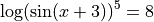
Find the solutions to

> let eqn1 = log(sin (x+3))^5 == 8 ;
> let sol1 = simplify $ solve eqn1 x;

The variable sol1 now contains an entire list of solutions. How many are there?

> #sol1 ;
10

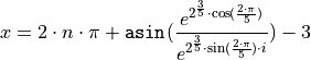
The first one is:

> sol1!0;
x==2*arbint 5*pi+asin (e^(2^(3/5)*cos (2*pi/5))/e^(2^(3/5)*sin (2*pi/5)*i))-3

where n is an arbitrary integer constant (shown as arbint 5 in the result of simplify).

It is also possible to obtain the right-hand side of any solution in the list via REDUCE commands:

> simplify $ rhs $ first $ solve eqn1 x;
2*arbint 10*pi+asin (e^(2^(3/5)*cos (2*pi/5))/e^(2^(3/5)*sin (2*pi/5)*i))-3

where first gets the first solution in the list and rhs obtains the right-hand side. Hence there is a wealth of possibilities to process the solution list.

Example 2:

Here are some simpler examples for the sake of clarity:

> simplify $ solve [X^2+1==0] X;
[X==i,X==-i]

> simplify $ solve [x+3*y==7,y-x==1] [x,y] ;
[[x==1,y==2]]

To get the multiplicities, turn on the switch multiplicities:

> simplify $ solve [x^2==2*x-1] x;
[x==1]
> reduce::switch "multiplicities" 1;
0
> simplify $ solve [x^2==2*x-1] x;
[x==1,x==1]

For details consult the REDUCE user manual.

Even and Odd Operators

An operator can be declared to be even or odd in its first argument by the declarations EVEN and ODD respectively.

> declare operator [f1,f2];
[]
> declare odd f1;
[]
> declare even f2;
[]

> simplify $ f1(-a);
-f1 a

> simplify $ f2 (-a);
f2 a

> simplify $ f1 (-a) (-b);
-f1 a (-b)

Linear Operators

An operator can be declared to be linear in its first argument over powers of its second argument.

> declare operator L;
[]
> declare linear L;
[]
> simplify $ L (a*x^5+b*x+c) x ;
L (x^5) x*a+L x x*b+L 1 x*c

> simplify $ L (a+b+c+d) y;
L 1 y*a+L 1 y*b+L 1 y*c+L 1 y*d

Note that L x y binds stronger than (*) in Pure.

Non-commuting Operators

An operator can be declared to be non-commutative under multiplication by the declaration NONCOM.

> declare operator [u,v];
[]
> simplify (u(x)*u(y)-u(y)*u(x));
0
> declare noncom [u,v];
[]
> simplify (u(x)*u(y)-u(y)*u(x));
u x*u y-u y*u x

Symmetric and Antisymmetric Operators

An operator can be declared to be symmetric with respect to its arguments by the declaration SYMMETRIC. Similarly, the declaration ANTISYMMETRIC declares an operator antisymmetric.

> declare operator [A,S];
[]
> declare symmetric S;
[]
> declare antisymmetric A;
[]

> simplify $ A x x ;
0

> simplify $ (A x y z) + (A x z y) ;
0

> simplify $ S y x ;
S x y

> simplify $ A y x ;
-A x y

Creating/Removing Variable Dependencies

There are several facilities in REDUCE, such as the differentiation operator and the linear operator facility, which can utilize knowledge of the dependencies between various variables. Such dependencies may be expressed by the command DEPEND.

> declare operator D ;
[]
> declare depend [D,x,y];
[]

> simplify $ df D a;
0

D does not depend on a, thus differentiating with respect to a yields 0, but

> simplify $ df D x;
df D x

because D is declared to depend on x. If we also let a depend on x, then:

> declare depend [a,x];
[]
> simplify $ df (D*a) x;
df D x*a+df a x*D

Note: Dependencies remain active until they are explicitly removed:

> declare nodepend [a,x];
> simplify $ df a x;
0
> simplify $ df (D*a) x;
df D x*a

Internal Order of Variables

It is possible for the user to change the internal order of variables by means of the declaration KORDER. The syntax for this is:

declare korder [v1,...,vn]

Unlike the ORDER declaration, which has a purely cosmetic effect on the way results are printed, the use of KORDER can have a significant effect on computation time.

> declare korder [z,y,x];
[]
> x+y+z;
x+y+z
> simplify $ x+y+z;
z+y+x

Parts of Algebraic Expressions

The following operators can be used to obtain a specific part of an expression, or even change such a part to another expression.

coeff expr::polynomial var

coeffn expr::polynomial var n::int

part expr::algebraic [n::int]

Examples:

> simplify $ coeff ((y^2+z)^3/z) y ;
[z^2,0,3*z,0,3,0,1/z]

> simplify $ coeffn ((y^2+z)^3/z) y 6;
1/z

> simplify $ part (a+b) 2 ;
b

> simplify $ part (a+b) 1 ;
a

> simplify $ part (a+b) 0 ;
(+)

PART may also be used to substitute a given part of an expression. In this case, the PART construct appears on the left-hand side of an assignment statement (cf. Assignment), and the expression to replace the given part on the right-hand side.

>  simplify $ xx:=a+b;
a+b
>  simplify $ part xx 2 := c ;
c
>  simplify $ xx;
a+c

Polynomials and Rationals

REDUCE is capable of factorizing univariate and multivariate polynomials with integer coefficients, finding all factors with integer coefficients. The package for doing this was written by Dr. Arthur C. Norman and Ms. P. Mary Ann Moore at The University of Cambridge. It is described in [SYMSAC81].

factorize expr::polynomial [p::prime]

Some examples:

> simplify $ factorize (x^105-1) ;
[[x^48+x^47+x^46-x^43-x^42-2*x^41-x^40 ... ]

> reduce::switch "ifactor" 1;
0
> simplify $ factorize (12*x^2 - 12) ;
[[2,2],[3,1],[x+1,1],[x-1,1]]
> reduce::switch "ifactor" 0;
0

The following operators should be well known:

gcd expr1::polynomial expr2::polynomial -> polynomial

lcm expr1::polynomial expr2::polynomial -> polynomial

remainder expr1::polynomial expr2::polynomial -> polynomial

resultant expr1::polynomial expr2::polynomial var -> polynomial

decompose expr::polynomial -> list

interpol <values> <variable> <points>) -> polynomial

deg expr::polynomial var ->int

den expr::rational -> polynomial

lcof expr::polynomial var -> polynomial

lpower expr::polynomial var-> polynomial

lterm expr::polynomial var -> polynomial

mainvar expr::polynomial -> expr

num expr::rational -> polynomial

reduct expr::polynomial var -> polynomial

Some examples of each operator:

GCD/LCM

> simplify $ gcd (x^2+2*x+1) (x^2+3*x+2) ;
x+1
> simplify $ gcd (2*x^2-2*y^2) (4*x+4*y) ;
2*x+2*y
> simplify $ gcd (x^2+y^2) (x-y) ;
1

> simplify $ lcm (x^2+2*x+1) (x^2+3*x+2) ;
x^3+4*x^2+5*x+2
> simplify $ lcm (2*x^2-2*y^2) (4*x+4*y) ;
4*x^2-4*y^2

REMAINDER/RESULTANT

> simplify $ remainder ((x+y)*(x+2*y)) (x+3*y) ;
2*y^2
> simplify $ remainder (2*x+y) 2 ;
y

> simplify $ resultant (x/r*u+y) (u*y) u ;
-y^2

DECOMPOSE

> simplify $ decompose (x^8-88*x^7+2924*x^6-43912*x^5+263431*x^4-
>                       218900*x^3+65690*x^2-7700*x+234) ;
[u^2+35*u+234,u==v^2+10*v,v==x^2-22*x]

> simplify $ decompose (u^2+v^2+2*u*v+1) ;
[w^2+1,w==u+v]

DEG/DEN

> simplify $ deg ((a+b)*(c+2*d)^2) d ;
2
> simplify $ deg ((x+b)*(x^6+2*y)^2) x ;
13

> simplify $ den (x/y^2) ;
y^2

LCOF/LPOWER/LTERM

> simplify $ lcof ((a+b)*(c+2*d)^2) a ;
c^2+4*c*d+4*d^2
> simplify $ lcof ((a+b)*(c+2*d)^2) d ;
4*a+4*b
> simplify $ lcof ((a+b)*(c+2*d)) ('e) ;
a*c+2*a*d+b*c+2*b*d

> simplify $ lpower ((a+b)*(c+2*d)^2) a ;
a
> simplify $ lpower ((a+b)*(c+2*d)^2) d ;
d^2
> simplify $ lpower ((a+b)*(c+2*d)) x ;
1

> simplify $ lterm ((a+b)*(c+2*d)^2) a ;
a*c^2+4*a*c*d+4*a*d^2
> simplify $ lterm ((a+b)*(c+2*d)^2) d ;
4*a*d^2+4*b*d^2
> simplify $ lterm ((a+b)*(c+2*d)) x ;
a*c+2*a*d+b*c+2*b*d

MAINVAR/NUM/REDUCT

> simplify $ mainvar ((a+b)*(c+2*d)^2) ;
a
> simplify $ mainvar 2 ;
0

> simplify $ num (x/y^2) ;
x
> simplify $ num ('(100/6)) ;
50
> simplify $ num (a/4+b/6) ;
3*a+2*b

> simplify $ reduct ((a+b)*(c+2*d)) a ;
b*c+2*b*d
> simplify $ reduct ((a+b)*(c+2*d)) d ;
a*c+b*c
> simplify $ reduct ((a+b)*(c+2*d)) x ;
0

Substitution

An important class of commands in REDUCE define substitutions for variables and expressions to be made during the evaluation of expressions. One such operation is the prefix operator SUB.

sub <substlist> exprn::algebraic -> algebraic

> simplify $ sub [x==a+y,y==y+1] (x^2+y^2) ;
a^2+2*a*y+2*y^2+2*y+1

> simplify $ sub [a==sin x, b==sin y] (a^2+b^2) ;
sin x^2+sin y^2

Note that simple substitutions of this kind can also be done directly in Pure, using the reduce macro.

Assignment

One may assign values to variables in the REDUCE environment. Note that in Pure the set operator and := are equivalent, i.e. both sides are evaluated, contrary to the := version in REDUCE.

set expr expr

expr := expr

> simplify $ P := a*x^n + b* x^m + c ;      // P:=a*x^n + b* x^m + c;
x^m*b+x^n*a+c
> simplify P ;                              // return P (from Reduce)
x^m*b+x^n*a+c
> simplify $ df P x;                        // diff P x
(x^m*b*m+x^n*a*n)/x
> simplify $ Q := intg P x ;                // integrate P x, store in Q
(x^m*b*n*x+x^m*b*x+x^n*a*m*x+x^n*a*x+c*m*n*x+c*m*x+c*n*x+c*x)/(m*n+m+n+1)

> simplify $ set Q (a*x^n + b* x^m + c) ;
x^m*b+x^n*a+c

Matrix Calculations

A very powerful feature of REDUCE is the ease with which matrix calculations can be performed. It fits very well into Pure’s native matrix type.

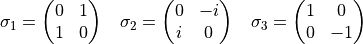
To keep it simple we show the usage of the different operators by examples using the well known Pauli matrices. See, e.g., http://en.wikipedia.org/wiki/Pauli_matrices for a reference.

let s0 = {1,0;0,1} ;
let s1 = {0,1;1,0} ;
let s2 = {0,-i;i,0};
let s3 = {1,0;0,-1};

Check the identities

where denotes the unit matrix.

Note: Instead of s1*s1 we could also write s1^2 here.

> let r1 = simplify $ (s1*s1) ; r1;
{1,0;0,1}
> let r2 = simplify $ (s2*s2) ; r2;
{1,0;0,1}
> let r3 = simplify $ (s3*s3) ; r3;
{1,0;0,1}
> let r4 = simplify $ (-i*s1*s2*s3) ; r4;
{1,0;0,1}
> let r5 = all (==s0) [r1,r2,r3,r4] ; r5;
1

Check:

> map (simplify . det) [s1,s2,s3] ;
[-1,-1,-1]

Calculate the eigenvalues/-vectors of :

> let r7 = simplify $ mateigen s2 q; r7;
[[q-1,1,{-c1*i;c2}],[q+1,1,{c3*i;c4}]]

> let r8 = map head r7; r8; // -> [q-1,q+1] => Eigenvalues q=+/-1
[q-1,q+1]

> let r9 = map (head.tail) r7 ; r9; // multiplicities
[1,1]

> let r10 = map last r7 ; r10; // eigenvectors
[{-c1*i;c2},{c3*i;c4}]

Transpose (operator tp):

> map (simplify.tp) [s1,s2,s3] ; // -> [s1',s2',s3']
[{0,1;1,0},{0,i;-i,0},{1,0;0,-1}]

Trace (operator trace):

> map (simplify.trace) [s1,s2,s3] ;
[0,0,0]

Cofactor (trivial here):

> simplify $ cofactor s2 1 1 ;
0

Nullspace of + {0,i;0,0}:

> simplify $ nullspace (s2+{0,i;0,0}) ;
[{0;1}]

Rank:

> map (simplify . rank) [s0,s1,s2,s3] ;
[2,2,2,2]

Inverse (simply ):

> let r15 = simplify $ 1/s2 ; r15;
{0,1/i;(-1)/i,0}

> simplify $ s2*r15 ;
{1,0;0,1}

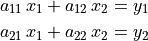
Solving without solve:

> simplify $ (1/{a11,a12;a21,a22}*{y1;y2}) ; // A^-1 * y' ;
{(-a12*y2+a22*y1)/(a11*a22-a12*a21);(a11*y2-a21*y1)/(a11*a22-a12*a21)}

Limits

From the package description:

LIMITS is a fast limit package for REDUCE for functions which are continuous except for computable poles and singularities, based on some earlier work by Ian Cohen and John P. Fitch. This package defines a LIMIT operator, called with the syntax:

limit expr::alg var limpoint::alg -> alg

> simplify $ limit (x*sin(1/x)) x infinity ;
1

> simplify $ limit (1/x) x 0 ;
inf

Notes: This package loads automatically. Author: Stanley L. Kameny.

Ordinary differential equations solver

The ODESOLVE package is a solver for ordinary differential equations.

Problem 1:

> declare depend [y,x];  // declare: y depends on x
[]

> simplify $ odesolve [df y x == x^2+exp(x)] [y] x ;
[y==(3*C+3*e^x+x^3)/3]

Problem 2:

> simplify $ odesolve [(df y x 2) == y] [y] x [[x==0,y==A],[x==1,y==B]] ;
[y==(-e^(2*x)*A+e^(2*x)*B*e+A*e^2-B*e)/(e^x*e^2-e^x)]

Remember to remove dependencies:

> declare nodepend [y,x];
[]

Series Summation and Products

SUM: A package for series summation

From the package description:

The package implements the Gosper algorithm for the summation of series. It defines operators SUM and PROD. The operator SUM returns the indefinite or definite summation of a given expression, and PROD returns the product of the given expression. This package loads automatically. Author: Fujio Kako.

Calculate

> simplify $ sum (n^3) n 1 N ;
(N^4+2*N^3+N^2)/4

> simplify $ sum (a+k*r) k 0 (n-1) ;
(2*a*n+n^2*r-n*r)/2

> simplify $ sum (1/((p+(k-1)*q)*(p+k*q))) k 1 (n+1) ;
(n+1)/(n*p*q+p^2+p*q)

> simplify $ prod (k/(k+2)) k 1 N ;
2/(N^2+3*N+2)

Taylor Series

TAYLOR: Manipulation of Taylor series

From the package description:

This package carries out the Taylor expansion of an expression in one or more variables and efficient manipulation of the resulting Taylor series. Capabilities include basic operations (addition, subtraction, multiplication and division) and also application of certain algebraic and transcendental functions. Author: Rainer Schöpf.

Example:

For details consult the package documentation in the REDUCE distribution.

> simplify $ taylor (exp (x^2+y^2)) x 0 2 y 0 2 ;
x^2*y^2+x^2+y^2+1

> simplify $ taylor (exp x) x 0 3;
(x^3+3*x^2+6*x+6)/6

> simplify $ implicit_taylor (x^2+y^2-1) x y 0 1 5 ;
(-x^4-4*x^2+8)/8

> simplify $ inverse_taylor (exp(x)-1) x y 0 8;
(-105*y^8+120*y^7-140*y^6+168*y^5-210*y^4+280*y^3-420*y^2+840*y)/840

Note that the “big O” residual terms are omitted in the results returned by simplify, although REDUCE will print them.

Boolean Expressions

The truth values within REDUCE are t and nil = (). Not all predicates (functions returning a truth value) can be called by simplify, however, so one has to use the lisp function in some circumstances.

Some examples:

> simplify $ evenp 200 ;
t
> simplify $ evenp 201 ;
[]

> lisp (fixp 200) ;
t

where fixp tests for integers.

The following example shows a pitfall. Since there is a numberp function in both Pure and REDUCE, the function needs to be quoted to make the expression go through to REDUCE:

> lisp (numberp x) ;
0
> lisp (numberp 111) ;
1

> lisp ('numberp x) ;
[]
> lisp ('numberp 111) ;
t

In the first case numberp x evaluates to zero in Pure, so the lisp function gets 0 and returns 0. In the second case (quoted) the function numberp is evaluated in REDUCE and returns nil, i.e. [] in Pure. Of course, both results are correct but there may be other cases where equally named functions have different meanings in the two environments.

Some other useful predicates in REDUCE are ordp and freeof:

> lisp (ordp x y) ;
t
> lisp (ordp y x) ;
[]
> lisp (ordp "abc" "abd") ;
t
> lisp (ordp "abd" "abc") ;
[]
> lisp (ordp 3 5) ;
[]
> lisp (ordp 5 3) ;
t

> simplify $ freeof (x^2+y) x ;
0
> simplify $ freeof (x^2+y) z ;
1
> simplify $ freeof (x^n*y^m) (y^m) ;
0

Mathematical Functions

REDUCE provides many mathematical functions which can take arbitrary scalar expressions as their single argument:

• ACOS ACOSH ACOT ACOTH ACSC ACSCH ASEC ASECH ASIN ASINH
• ATAN ATANH ATAN2 COS COSH COT COTH CSC CSCH DILOG EI EXP
• HYPOT LN LOG LOGB LOG10 SEC SECH SIN SINH SQRT TAN TANH ERF

Note that Pure also defines some these functions in its math module, so these may have to be quoted to prevent evaluation on the Pure side. For instance:

> simplify $ cos 4.3;
cos (43/10)
> using math;
warning: external 'exp' shadows previous undefined use of this symbol
warning: external 'sin' shadows previous undefined use of this symbol
warning: external 'cos' shadows previous undefined use of this symbol
> simplify $ cos 4.3;
(-21601483)/53896027

Some examples:

> simplify $ cos (-x) ;
cos x
> simplify $ cos (n*pi) ;
cos (80143857*n/25510582)
> simplify $ (quote e)^(3*i*(quote pi)/2) ;
-i
> simplify $ sec (quote pi);
-1
> let simplify $ log10 10 ;
1
> simplify $ erf (-a);
-erf a

The special functions are in two separate packages SPECFN and SPECFN2:

• Bernoulli Numbers and Euler Numbers;
• Stirling Numbers;
• Binomial Coefficients;
• Pochhammer notation;
• The Gamma function;
• The Psi function and its derivatives;
• The Riemann Zeta function;
• The Bessel functions J and Y of the first and second kind;
• The modified Bessel functions I and K;
• The Hankel functions H1 and H2;
• The Kummer hypergeometric functions M and U;
• The Beta function, and Struve, Lommel and Whittaker functions;
• The Airy functions;
• The Exponential Integral, the Sine and Cosine Integrals;
• The Hyperbolic Sine and Cosine Integrals;
• The Fresnel Integrals and the Error function;
• The Dilog function;
• Hermite Polynomials;
• Jacobi Polynomials;
• Legendre Polynomials;
• Spherical and Solid Harmonics;
• Laguerre Polynomials;
• Chebyshev Polynomials;
• Gegenbauer Polynomials;
• Euler Polynomials;
• Bernoulli Polynomials.
• Jacobi Elliptic Functions and Integrals;
• 3j symbols, 6j symbols and Clebsch Gordan coefficients;

In SPECFN2 are the generalized hypergeometric functions and Meijer’s G function.

Author: Chris Cannam, with contributions from Winfried Neun, Herbert Melenk, Victor Adamchik, Francis Wright and several others.

Definite Integrals

DEFINT: Calculating definite integrals by using the Meijer G integration formula.

> reduce::load "defint" ;
0

> simplify $ intg (exp(-x)) x 0 infinity ;
1

> simplify $ intg (x^2*cos(x)*exp(-2*x)) x 0 infinity ;
4/125

> simplify $ intg (x*exp(-1/2*x)) x 0 1 ;
2*sqrt e*(2*sqrt e-3)/e

> simplify $ intg (x*log(1+x)) x 0 1 ;
1/4

> simplify $ intg (cos(2*x)) x y (2*y);
(sin (4*y)-sin (2*y))/2

Various transformations:

> simplify $ laplace_transform (exp(-a*x)) x ;
1/(a+s)

> simplify $ hankel_transform (exp(-a*x)) x ;
s^(n/2)*gamma (n/2)*hypergeometric [(n+2)/2] [n+1]
((-s)/a)*n/(2*a^(n/2)*gamma (n+1)*a)

> simplify $ y_transform (exp(-a*x)) x ;
(a^n*gamma (n+1)*gamma ((-n)/2)*gamma ((-2*n-1)/2)*gamma
((2*n+3)/2)*hypergeometric [(-n+2)/2] [-n+1] ((-s)/a)+s^n*gamma
(-n)*gamma (n/2)*hypergeometric [(n+2)/2] [n+1] ((-s)/a)*n*pi)/
(2*s^(n/2)*a^(n/2)*gamma ((-2*n-1)/2)*gamma ((2*n+3)/2)*a*pi)

> simplify $ k_transform (exp(-a*x)) x ;
(-a^n*gamma (n+1)*gamma ((-n)/2)*hypergeometric [(-n+2)/2] [-n+1]
(s/a)+s^n*gamma (-n)*gamma (n/2)*hypergeometric [(n+2)/2] [n+1] (s/a)*n)/
(4*s^(n/2)*a^(n/2)*a)

>  simplify $ struveh_transform (exp(-a*x)) x ;
2*s^((n+1)/2)*gamma ((n+3)/2)*hypergeometric [1,(n+3)/2] [(2*n+3)/2,3/2]
((-s)/a)/(sqrt pi*a^((n+1)/2)*gamma ((2*n+3)/2)*a)

> simplify $ fourier_sin (exp(-a*x)) x ;
s/(a^2+s^2)
> simplify $ fourier_cos (exp(-a*x)) x ;
a/(a^2+s^2)

Declarations, Switches and Loading

Lisp evaluation can be used in the REDUCE system, in particular, to declare operator symbols and their properties (simplify won’t do that). E.g.:

> lisp ('operator [myop]);
> lisp ('flag [myop] odd);
> lisp ('prop myop); // => [odd:t,simpfn:simpiden]
> simplify (myop (-x)); // => -myop x

For the most common kinds of declarations, the reduce module provides the declare function which takes care of the necessary Lisp magic and is safe to use. The above example can also be done as follows:

> declare operator myop;
> declare odd myop;
> simplify (myop (-x));
-myop x

Please see the description of declare for a list of supported declarations.

The reduce module also provides a few other basic maintenance functions which are done with special commands in REDUCE:

reduce::switch "switch-name" 0|1

reduce::load "package-name"

reduce::in "path/filename.red"

reduce::capture 0|1

reduce::feed "text"

As already mentioned, REDUCE switches can be turned on and off with reduce::switch, e.g.:

> reduce::switch "exp" 0 ;
0

Packages can be loaded with the reduce::load command:

> reduce::load "defint" ;
0

REDUCE source files can be read in with the reduce::in command:

> reduce::in "myreduce.red" ;
0

Last but not least, REDUCE terminal input and output can also be redirected to string buffers using the reduce::feed and reduce::capture functions. For instance, the following code feeds some text with a Lisp form to REDUCE, which gets read by evaluating the Lisp form (eval read). The output is captured and can be inspected with the reduce::output function:

> reduce::feed "(print '(a b c d))";
0
> reduce::capture 1; // start capturing output
0
> lisp ('eval read); // read buffered input and evaluate
[a,b,c,d]
> reduce::output;    // inspect buffered output
"(a b c d)\n"
> reduce::capture 0; // stop capturing output
0

Plotting

REDUCE can do 2- and 3-dimensional function plots through its gnuplot package. Some examples (note that we have to quote the x..y ranges here so that they get through to Reduce, rather than being evaluated on the Pure side):

> simplify $ plot (sin x/x) (x=='(-15..15));

// Multiple ranges.
> simplify $ plot (sin(x^2 + y^2) / sqrt(x^2 + y^2)) [x=='(-12..12), y=='(-12..12)];

// Specifying options.
> simplify $ plot (cos (sqrt(x^2 + y^2))) [x=='(-3..3),y=='(-3 .. 3)] hidden3d;

// Specifying points.
> simplify $ plot [[0,0],[0,1],[1,1],[0,0],[1,0],[0,1],[0.5,1.5],[1,1],[1,0]];

// Output options.
> simplify $ plot (sin x) [x=='(0..10),terminal==postscript,output=="sin.ps"];

References

[REDUM]

REDUCE User’s Manual, Version 3.8, Anthony C. Hearn, Santa Monica, CA, USA.

[LNCS102]

On the Integration of Algebraic Functions, LNCS 102, Springer Verlag, 1981.

[SYMSAC81]

P. M. A. Moore and A.C. Norman, Implementing a Polynomial Factorization and GCD Package, Proc. SYMSAC ’81, ACM (New York) (1981), 109-116.